Understanding Happiness Metrics: An Analytical Approach
Written on
Chapter 1: Introduction to Happiness Analysis
Recent research has demonstrated that happiness is quantifiable. A team of leading researchers conducted a widespread survey across nearly 150 nations to pinpoint the happiest populations. In this analysis, we will delve into the data from their study and explore a critical question: Is financial wealth the sole determinant of happiness?
Prerequisites
To begin, familiarize yourself with the findings available on the World Happiness Report 2021 official website. Afterward, download the dataset and prepare your coding environment.
Features of the Dataset
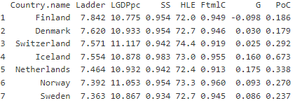
The dataset comprises seven numerical columns that capture various aspects of societal development:
- Ladder score (Ladder)
- Logged GDP per capita (LGDpc)
- Social security (SS)
- Healthy life expectancy (HLE)
- Freedom to make life choices (FtmlC)
- Generosity (G)
- Perception of corruption (PoC)
It's important to note that these features may show negative values. For instance, Finland's population exhibited a slight increase in greed compared to the previous year.
Chapter 2: Visualizing Happiness Data
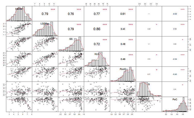
Super-Scatterplot
Imagine combining histograms, kernel density functions, and mini-scatterplots into one comprehensive super-scatterplot.
Correlation Heatmap
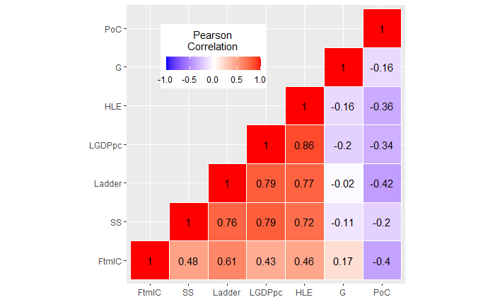
A sophisticated method to display a correlation matrix is through a heatmap. Here, we utilized a hierarchical clustering algorithm to create groups that are visually appealing.
Correlation Graph
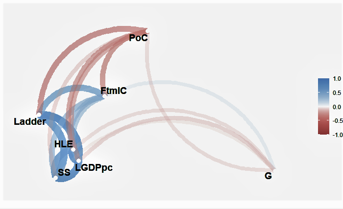
Employing topological techniques, we can transform numerical data into a two-dimensional representation.
Comparative Analysis of Correlation Coefficients
The Pearson correlation coefficient (CC) provides a parametric method to assess the strength of relationships between variables.
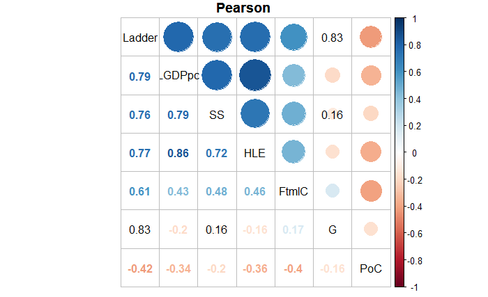
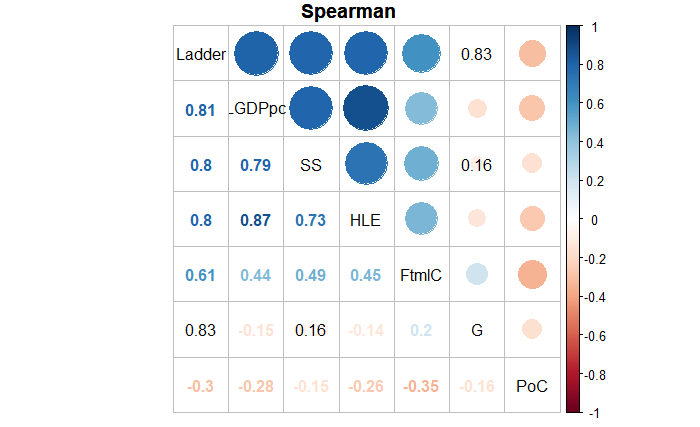
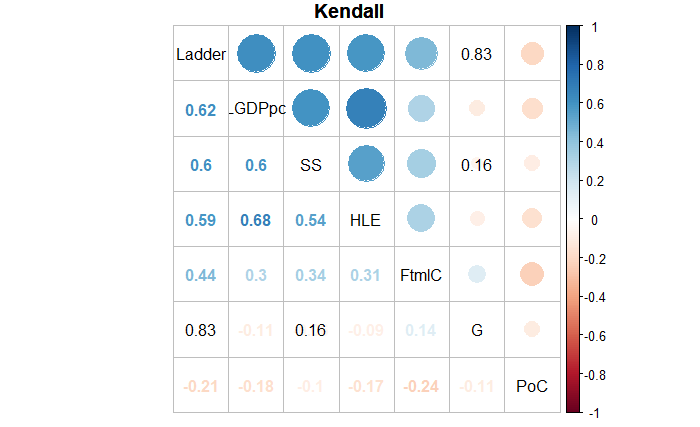
Meanwhile, Spearman and Kendall coefficients introduce ranking for evaluating continuous or categorical variables, focusing on monotonicity rather than linearity.
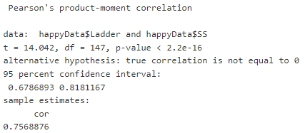
Pearson Correlation Test
Let's compute the Pearson correlation coefficient between the Ladder score and Social Security metrics.
Understanding the Mathematics of the 95% Confidence Interval
The concept of a "95 percent confidence interval" is intricate. Let's dissect it further.
The calculation for the confidence interval surrounding Pearson's CC (denoted as r) is asymmetric due to the skewed distribution of r. For instance, if r = 0.95, the actual population correlation cannot exceed 1.0 but could be significantly lower.
The confidence interval is derived from Fisher’s z transformation. Given a sample of n pairs producing an r value, the transformation is expressed as follows:
In this context, z is approximately normally distributed with an expected value equal to...

Confidence intervals can be established in z-space, which allows us to translate back to r-space.
Calculating the upper and lower limits of the confidence interval in z-space leads to the following results:

By inverting Fisher's z transform, we can determine the confidence interval limits in r-space.
Thus, for our analysis with n=149 and r=0.756, the 95% confidence interval ranges from 0.68 to 0.815.
Conclusion
This article provides a concise overview of a potent statistical method for data analysis and visualization—correlation. Additionally, it clarifies the mathematics underpinning the confidence interval of the Pearson correlation coefficient. Ultimately, happiness is influenced by more than just financial factors.
The first video titled "Text Analytics with R | Sentiment Analysis with R | Part 1 | Basics" offers foundational insights into sentiment analysis in R, setting the stage for our understanding of data interpretation.
The second video, "World Happiness Report 2021 Data Analysis Using Python," delves into the practical application of Python for analyzing happiness metrics, complementing the analytical methods discussed here.
The source code referenced in this article can be found here.