Understanding Systems of Linear Equations

Equations 1–3 illustrate a typical set of linear equations. A "system" indicates that there may be shared solutions among the equations. The term "linear" refers to the fact that the highest exponent of the unknown variables, such as x₁, x₂, and x₃, is one.

The Gaussian elimination algorithm seeks to determine values for x₁, x₂, and x₃ that satisfy all equations simultaneously. This method is frequently employed in computing to efficiently evaluate numerous variables.

To define the symbolic system of equations, utilize the Python code provided in Gist 1, which employs the Sympy library.

Algorithm Overview

Gaussian elimination relies on matrix algebra. Begin by expressing Equations 1–3 in matrix format, Ax = b, as shown in Equation 4.

• The coefficients of the variables are included in matrix A.
• The unknowns x₁, x₂, and x₃ are represented as a column vector x.
• The column vector b comprises the right-hand sides of the equations.

By multiplying the rows of A with the x column vector, the original equations can be retrieved. Next, form the augmented matrix, which concatenates matrix A with matrix b on the right side, as depicted in Equation 5.

Create the augmented matrix in Python using the code snippet from Gist 2. The matrix_representation function requires previously defined variables and symbolic representations.

Transitioning to Row Echelon Form

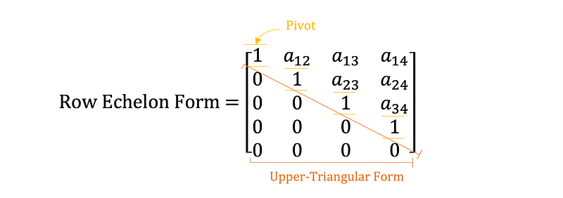
The next step is to convert the augmented matrix into row echelon form using Gaussian elimination. The characteristics of row echelon form are:

• The first non-zero row appears to the right of the leading coefficient in the row above, known as the pivot.
• Zeros are present below the diagonal, resulting in an upper-triangular matrix.
• Any rows filled entirely with zeros are positioned at the bottom of the matrix.

Equation 6 illustrates these concepts.

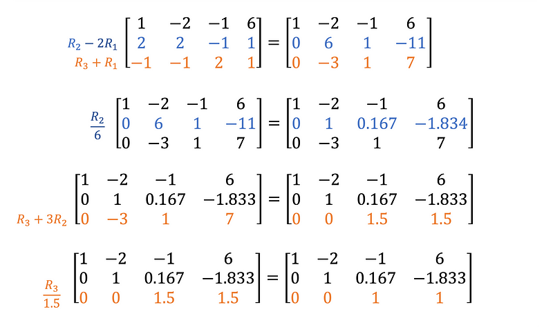
To achieve this form, specific row operations are applied, such as:

• Multiplying any row by a constant.
• Adding multiples of one row to another.
• Switching the order of any rows.

Continuing from the system shown in Equation 5, Equations 7–10 illustrate how to convert the augmented matrix into upper-triangular form.

Implement these row operations in code to transform any given augmented matrix M into upper-triangular form. Gist 3 provides a Python algorithm for performing Gaussian elimination and converting a system of Sympy symbolic equations into row echelon form.

After executing the code, printing M to the console yields an upper-triangular matrix represented as follows:

upper triangular matrix: [[ 1. -2. -1. 6. ]

[ 0. 1. 0.166667 -1.83334 ]

[ 0. 0. 1. 1. ]]

This upper-triangular matrix provides three simplified expressions involving x₁, x₂, and x₃, as illustrated in Equations 11–13.

Solving for Unknown Variables

Backward substitution allows for the resolution of the unknown variables:

• x₃ = 1.0: directly derived from Equation 13.
• x₂ = -2.0: found by substituting x₃ into Equation 12.
• x₁ = 3.0: determined by substituting both x₂ and x₃ into Equation 11.

Gist 4 demonstrates the code for performing back substitution to solve for the unknowns.

The Gaussian elimination algorithm has successfully determined the solutions to the system of linear equations through row reduction and back substitution, yielding results consistent with manual calculations:

solutions: [3.0000, -2.0000, 1.0000] # (x1, x2, x3)

Edge Cases in Gaussian Elimination

1. No solution: If the row echelon form includes a row of all zeros except for the right-hand side, the system is inconsistent. This situation can be represented by the contradiction 0 ≠ 1.

Inconsistent System:

[[ 1. 1. -3. 4.]

[-0. 1. -5. 6.]

[ 0. 0. 0. 1.]]

2. Infinite solutions: If there is a row of all zeros and the number of non-zero rows is fewer than the number of variables, the system is dependent, indicating an infinite number of solutions.

Dependent System:

[[ 1. 1. -3. 0.]

[-0. 1. -5. -0.]

[ 0. 0. 0. 0.]]

Visualizing the Solution

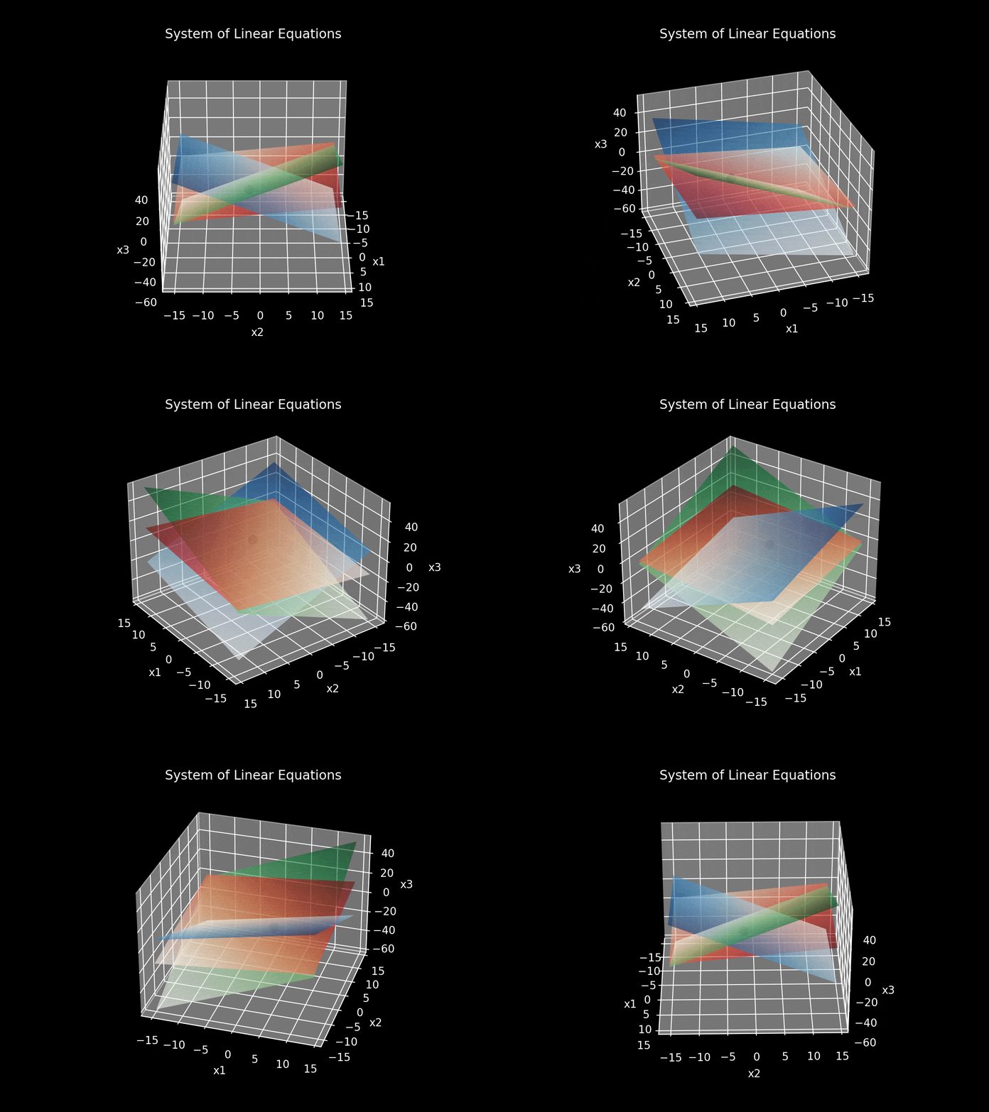
A linear equation with three unknowns represents a plane in three-dimensional space, with each variable corresponding to a distinct axis in a Cartesian coordinate system. Figure 1 depicts the planes formed by Equations 1–4:

• The blue plane corresponds to Equation 1: x₁ – 2 * x₂ – x₃ – 6 = 0
• The green plane corresponds to Equation 2: 2 * x₁ + 2 * x₂ – x₃ – 1 = 0
• The red plane corresponds to Equation 3: – x₁ – x₂ + 2 * x₃ – 1 = 0

The intersection point, which represents the solution to the system of three linear equations, is shown as a black dot at [3.0, -2.0, 1.0].

This coordinate point signifies the unique solution, aligning with the earlier algebraic results. Conversely, a graphical representation of a dependent system illustrates that the intersection of planes creates a line, resulting in an infinite number of solutions. An inconsistent system is depicted by three planes that do not intersect.

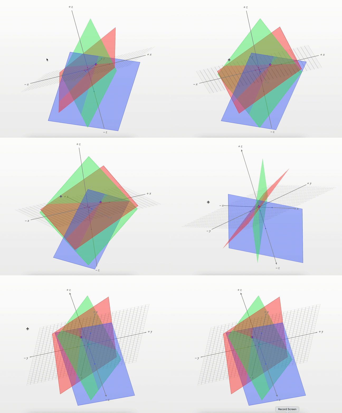
For a clearer visual representation of these scenarios, utilize this advanced graphing tool. Figure 2 showcases the same equations as Figure 1 but with enhanced graphics.

5 Python Projects for Engineering Students

Beginner to Intermediate Python Project Ideas for Engineers

References

[1] Row Echelon Form — The Unapologetic Mathematician (Mathematics for the interested outsider)

[2] Row reduction, row-echelon form, and reduced row-echelon form — Lorenzo Sadun (July 30th 2013)

[3] Systems of Equations in Three Variables — lumenlearning