Chapter 1: Introduction to Grid Paths

In this discussion, we will delve into the fascinating topic of paths on a two-dimensional grid. Below is a representation of what such a path might resemble:

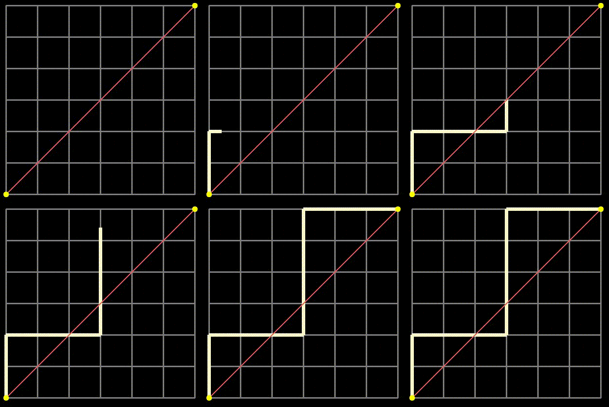
Fig 1: Examples of grid paths we will analyze.

We will explore how to count paths that meet specific criteria. While the sheer joy of counting can serve as motivation, there are additional practical reasons to engage with this topic. Consider how often you encounter a graph with x and y axes—such as a stock price chart where the x-axis represents time and the y-axis represents the stock price. Essentially, time series data often depicts these paths as grids, with the stock price moving either up or down at each step. This kind of motion is referred to as “Brownian motion,” which was initially used to describe the erratic movement of dust particles. Another analogy involves a gambler who flips a coin, gaining $1 for heads and losing $1 for tails. The grid paths illustrated above symbolize his cumulative profit over a series of coin flips, hence the term “gambler paths.”

These models are instrumental in pricing financial instruments linked to these stocks, such as options.

Next, we will examine the simplest scenario involving square grids. The total number of paths that only allow movement towards a target—meaning only upward or rightward steps as shown in Figure 1—is a concept taught in high school mathematics. Additionally, the famous Catalan numbers represent paths that adhere to these rules without crossing the main diagonal (the red line in Figure 1). It’s important to note that the path depicted in Figure 1 crosses this line twice, rendering it “invalid” under these constraints.

Following Theodore Sturgeon’s advice to “ask the next question,” we will analyze paths on rectangular grids, thereby generalizing our examination of square grids. This relates closely to “Bertrand’s ballot problem,” where candidate A receives p votes and candidate B receives q votes, and we seek the probability that candidate A was always in the lead after each vote. Lastly, we will revisit square grids but focus on paths that cross the main diagonal k times instead of never crossing it at all. When k=0, we should retrieve the original sequence. The concluding question will involve both generalizations—paths that traverse a rectangular grid while crossing a certain horizontal line k times. By the time we reach this stage, the solution will emerge quite intuitively.

1. Total Paths

Let’s begin with a straightforward scenario and consider the total paths from the bottom left to the top right of the grid, allowing only rightward and upward movements in the square grid of Figure 1. For an n×n grid, we need to make a total of 2n steps, comprising n steps to the right and n steps upward. Therefore, it simply becomes a matter of choosing which n of those 2n steps will be upward and which will be rightward. Consequently, the total number of such paths is given by {2n choose n}.

2. Dyck Paths

As mentioned earlier, the paths on the grid are useful for modeling time-series data (like stock prices). This can be visualized by dividing time into discrete intervals where the stock price either increases or decreases by one unit at each step on the grid. Initially, the connection between the path in Figure 1 and this concept may not be obvious, but it becomes clear once we rotate it, as shown in Figure 2 below.

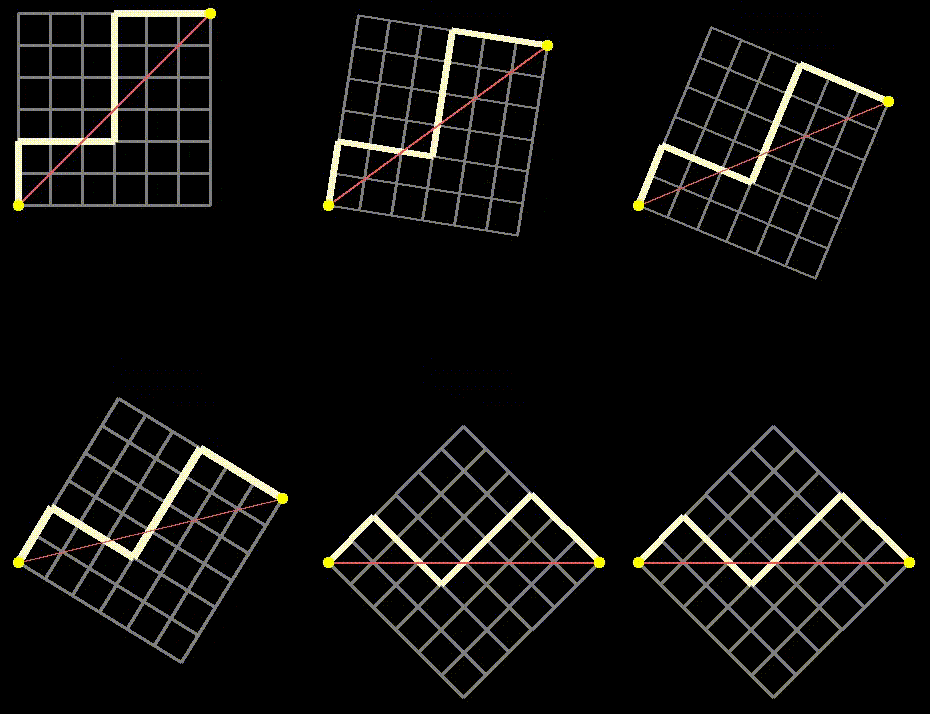
Fig 2: Rotated grid illustrating time-series paths.

The paths we will first analyze are those that start and end at y=0 (the two yellow points in Figure 3) while avoiding crossing the central red line illustrated in Figure 2. These paths are termed "Dyck paths," as they remain either above or below the x-axis. For each path that stays above, there exists a symmetric counterpart that remains below, as demonstrated in Figure 3.

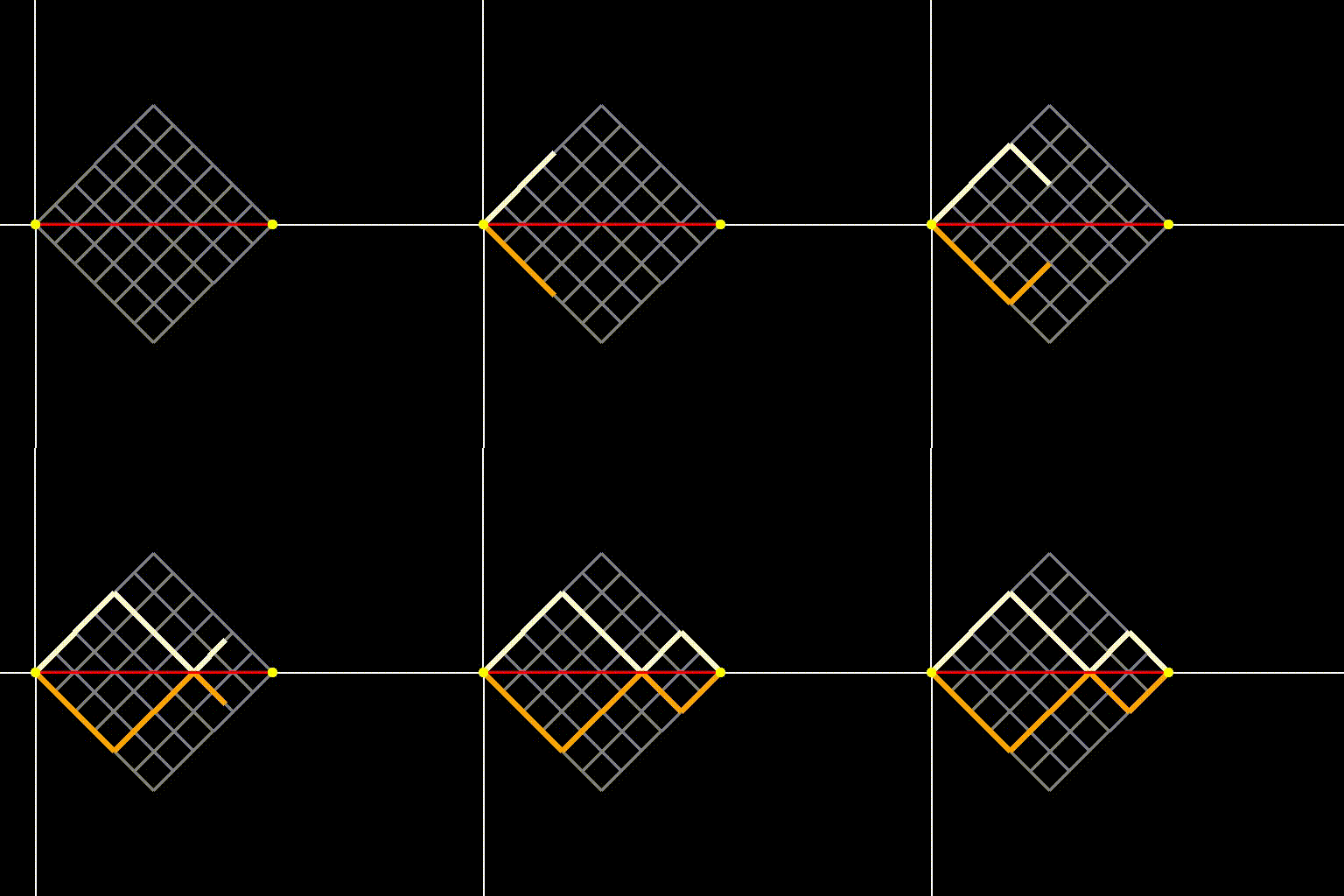
Fig 3: Dyck paths on a two-dimensional grid—they may touch but do not cross the red diagonal.

Since the paths begin and end at y=0, the number of upward steps must equal the number of downward steps. Thus, the total number of steps must be even, specifically 2n, where n denotes the side length of the square grid. Let’s denote the number of paths that remain below y=0 (like the orange path in Figure 3) in a grid of side n as c_n. In our analogy of the gambler flipping a coin, this signifies starting and ending at a balance of $0 without ever having a positive balance (or conversely, never going into negative balance).

We will compute c_n through two methods.

#### 2.1 Andre’s Reflection Method

We know that there are {2n choose n} total paths, but we need to exclude those that cross the main diagonal (the purple line in Figure 4).

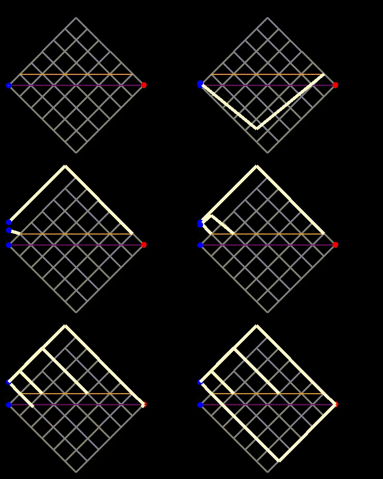
Fig 4: The reflection method where paths crossing the purple line and touching the orange line are mapped to paths on the yellow grid.

Now, since each undesirable path on the original grid corresponds to a path on the bright yellow grid, we can count the undesirable paths. The total paths on the bright yellow grid still require 2n steps, but with n-1 upward steps, leading to a total count of {2n choose n-1} for undesirable paths. Therefore, the number of valid paths (those that do not touch the main diagonal) is the total paths ({2n choose n}) minus the undesirable paths. This gives us the total paths that move from (0,0) to (n,n) without crossing the main diagonal, denoted by c_n:

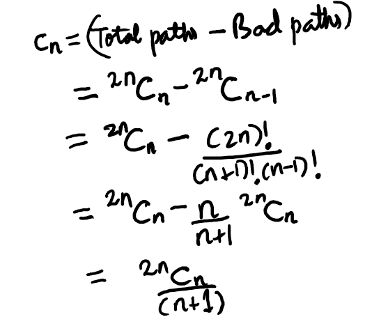
Eq (1): Counting the paths on an n-by-n grid that never cross the main diagonal and remain on one side.

2.2 Using a Recurrence

Next, we will present a path that is less visual but will ultimately provide a powerful tool applicable to a wide range of “paths on a grid” problems. This tool is the “generating function” of a sequence. Let’s first formulate a recurrence relation. Consider the number of paths that first touch the main diagonal (or x-axis) after a given number of steps from the starting point. To avoid touching it beforehand, we must initially take an upward step and reach the orange line in Figure 5 below.

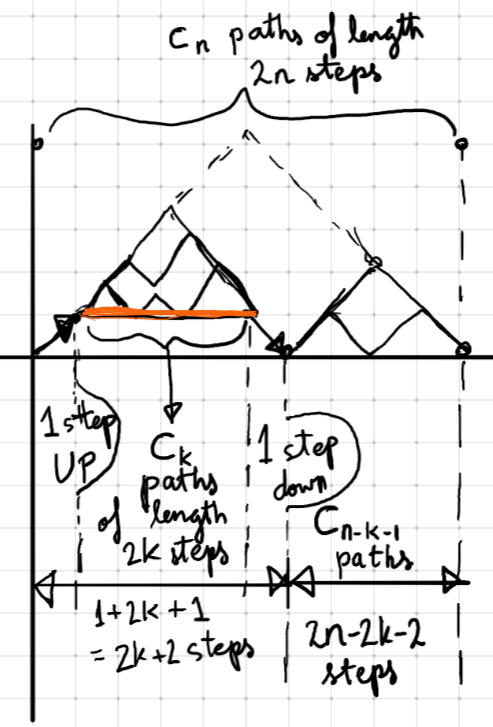
Fig 5: Paths on the grid where we take 2n steps (n-up and n-down), remaining at or above the x-axis.

Thus, if the orange path has a length of 2k, we first touch the main diagonal (or x-axis) at step 2k+2. The total paths that touch the main diagonal after 2k+2 steps while satisfying the original condition of remaining above it become: c_k × c_{n-k-1}. Here, k can take any value from 0 to n-1. Paths corresponding to k=0 and k=n-1 never touch the x-axis (or main diagonal) except at the beginning and end of their journeys. This leads us to the recurrence relation:

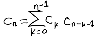
Eq (2): The recurrence expressing the number of paths in terms of itself.

This recurrence mirrors that found in exercise 12–4 of the book “Introduction to Algorithms” by Cormen et al., a widely regarded reference in computer science. This chapter discusses binary trees, which allow for various operations such as look-up, insertion, and deletion in O(log(n)) time. The inclusion of a recurrence related to paths on a grid in this chapter serves to illustrate the number of binary trees with one node reserved for the root, where every node has either zero or two children. The satisfaction of the same recurrence with equivalent starting conditions indicates that the sequences are identical, showing that the number of paths on a grid with n upward and n downward steps without crossing the main diagonal is equivalent to the number of binary trees with n nodes (both sequences represented by the Catalan numbers). A glance at the Wikipedia page on Catalan numbers reveals that numerous seemingly unrelated counting problems adhere to this sequence.

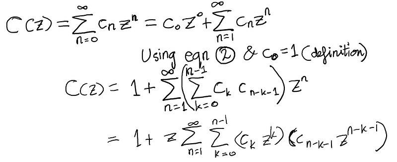
As we seek to use the recurrence to derive a closed-form solution for c_n, we begin by defining the generating function of the sequence c_n as follows:

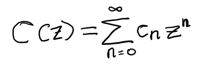
Eq (3): Definition of the generating function.

If we can express C(z) in a closed form, it may assist us in obtaining the expression for c_n by determining what the coefficient of z^n would yield if we represented it as a polynomial. We can substitute the recurrence from equation (2) into the generating function defined above.

3. Raising the Glass Ceiling

#### 3.1 Generalizing the Sequence of Paths

The Dyck paths discussed in section 2 always start and end at the same level (designated as level 0). However, real-life paths on a grid may not necessarily adhere to this constraint. A gambler might opt to cease tossing the coin at a certain level of profit or loss. Let’s take the grid we’ve been examining and elevate the target from returning to 0 to finishing at a profit of (for example) $4 (as represented by the orange line).

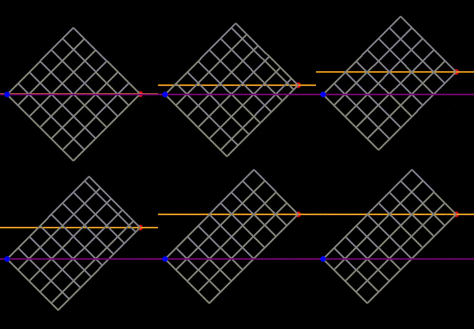
Fig 6: Analyzing general paths that do not necessarily terminate at the same vertical level as their starting point.

While we begin at the blue point and aim to reach the red point, the red point can now be positioned at a different vertical level than the blue point. The question becomes: how many paths extend from the blue point to the red point without crossing the orange line? This inquiry equates to determining how many ways the gambler can achieve $4 after flipping 8 heads and 4 tails without crossing $4 at any moment. First, note that this scenario is equivalent to counting paths where his balance remains non-negative (where he never crosses the purple line, indicating a $0 balance in the preceding figure). This relationship can be established by starting with a path that crosses the orange line and then rotating the entire grid, effectively reversing the path. This adjustment transforms it into a path that dips below the purple line, demonstrating a one-to-one mapping (or bijection) between the two types of paths.

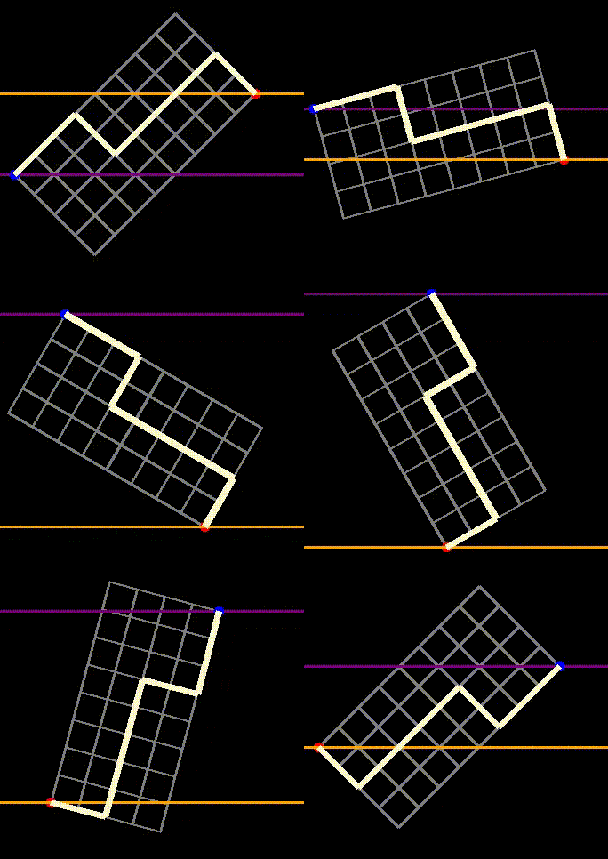
Fig 7: Demonstrating that paths crossing the purple line from above correspond to paths crossing the orange line from below.

Now, let’s determine the number of paths.

Definition-1: Let c_{l,t} denote the number of paths in which a gambler achieves t tails and t+l heads, culminating in a profit of l$ without ever crossing l$.

#### 3.2 The Reflection Method Revisited

We can apply Andre’s reflection method once more, employing a similar approach to that utilized in Figure 4. The process is illustrated in Figure 8, which shows the transition from the blue point to the red point while avoiding the orange line. If any aspect is unclear, please revisit section 2.1.

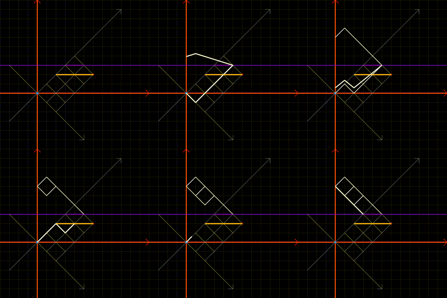
Fig 8: Andre’s reflection method applied to a rectangular grid.

Figure 8.1 provides a static representation of the reflection method. The steps involved include:

1. Reflect the origin (the blue point) across the purple line (y=l+1), where touching is impermissible.
2. Construct the yellow grid from the reflected blue point to the red point, representing the “undesirable paths” to exclude.
3. The height of the yellow grid is (t-1).

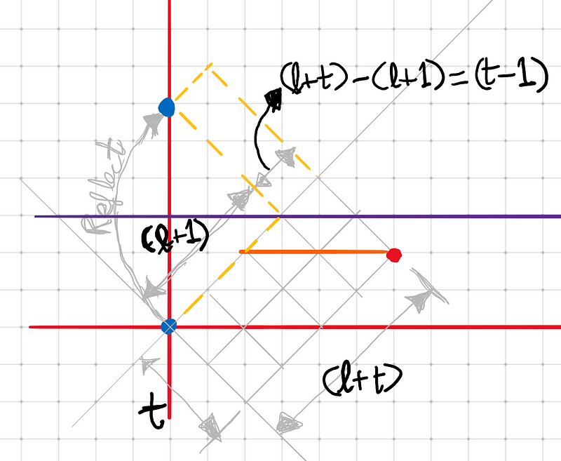
Fig 8.1: Static depiction of the reflection method with explanatory labels.

Given that the gambler requires (t+l) heads and t tails, the total paths are represented by {2t+l choose t}. Since the total steps needed in the yellow grid formed after reflection remains unchanged, we can derive the paths of interest:

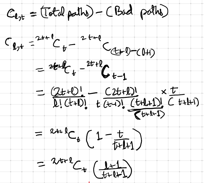
Eq 5.5: The closed-form expression for c_{l,t} utilizing Andre’s reflection method.

4.3 Generating Functions

Next, we will obtain the actual closed-form expression for c_{l,t} through generating functions. While the reflection method suffices for determining c_{l,t}, the generating function will provide a framework for addressing a more generalized version of the problem.

An alternative definition simplifies our task:

Definition-2: c_{l,t} also represents the number of ways to first reach (l+1)$ with t heads and t+l+1 tails.

Notice that in this second definition, touching the target (l+1)$ level before reaching it is not permitted, while the first definition allows touching l$ but not crossing it. Both definitions are equivalent since once reaching l$ with t tails and t+l heads, there is only one way to proceed to (l+1)$ in one additional toss: obtaining another heads and gaining another dollar.

Now, define the generating function for the sequence that characterizes the ways in which the gambler reaches l$:

Eq (6): Generating function for the sequence c_{l,t}.

4.3.1 Consolidating the Generating Functions

Notably, substituting l=0 into equation (6) yields C_0(z)=C(z) as defined in equation (3) and solved in equation (5). Can we express other C_l(z) in terms of C(z) as well? We can utilize a clever probability trick here. In this context, Definition-2 of c_{l,t} proves useful. Consider a gambler tossing a coin until he reaches $1. What’s the probability of him ever reaching that target? Let’s define this as event E. Define E_t as the event where he reaches $1 for the first time with exactly t tails (which necessitates (t+1) heads by that point). Thus, event E occurs if he reaches $1 for the first time with 0 tails (by tossing heads first), or with 1 tail, or with 2 tails, and so on:

Hanging Eqn:

Each of E_0, E_1, etc., represents mutually exclusive events (only one can hold true at any given time). Thus, the probability of event E becomes:

To illustrate, what would P(E_2) signify? It represents the number of paths leading to $1 with 2 tails and 3 heads for the first time on toss 5, multiplied by the probability of obtaining 2 tails and 3 heads. Emphasizing paths that reach $1 for the first time with 2 tails is essential; if he had reached $1 sooner (with just one tail), he wouldn’t have actually reached it with 2 tails, which is the essence of E_2. The same reasoning applies to reaching l$ instead of $1, resulting in the following relationship of these probabilities expressed through the generating functions defined in equation (6) (where p is the probability of the coin landing heads).

Eq (6.5): The probabilities of reaching $1 and l$ in terms of the generating functions, C_l(z).

4.3.2 Defining a Recurrence

Now, we can formulate a recurrence for the c_{l,t} terms by considering the gambler's first coin toss. Refer to Figure 9. Initially, the gambler is at the blue point, aiming for the red point at level l with t tails. If his first toss yields heads, he reaches the purple level. Here, he must ascend (l-1) levels to reach the red point, while still retaining t tails. Conversely, if his first toss is tails, he reaches the green level, where he must now ascend (l+1) levels to reach the red point while needing one less tail to succeed.

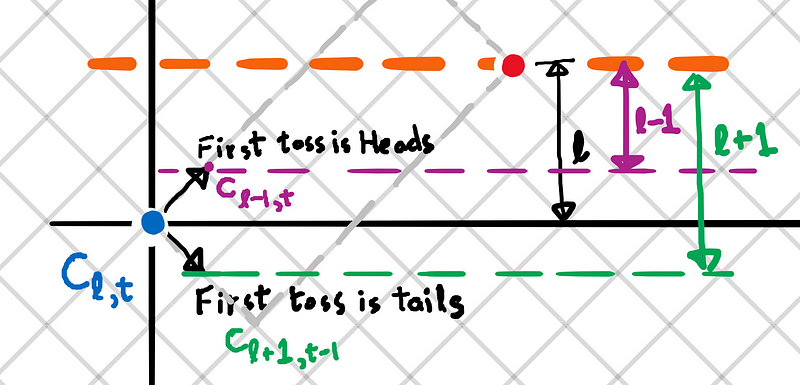
Fig (9): Recurrence for c_{l,t} based on the first toss.

As a result, we derive the recurrence:

Eq (8): Recurrence for c_{l,t} based on the first toss.

4.3.3 Solving the Recurrence

We can convert the recurrence for paths, c_{l,t}, into a recurrence for the generating function: C_{l}(z).

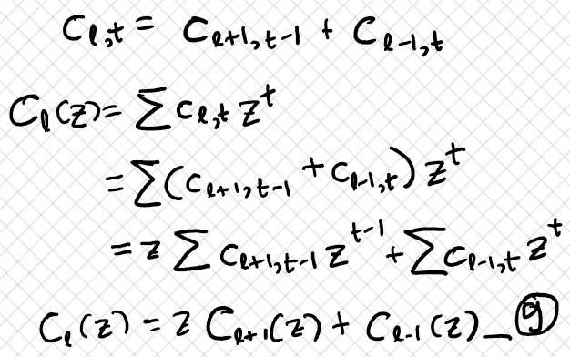
Eq (9): An expression for the generating function.

Next, we can utilize the relationship established from the probability trick in equation (7):

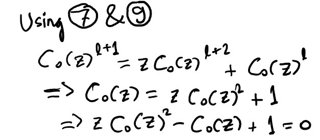
Eq (10): Deriving an expression for the recurrence.

This leads us back to the expression from equation (4). The solution to this, achieved by resolving the quadratic equation in C_0(z)=C(z), yields the solution presented in equation (5).

We already have the expression for C_0(z) and thus c_{0,t}. Our goal is to derive an expression for c_{l,t}. Starting with:

Since c_{-1,t}=0 by definition-2 (representing paths for the gambler reaching $0 for the first time with t tails), this counts as 0 because he starts at $0; thus, his path’s end won’t be the first instance he hits $0. Consequently, c_{1,t-1}=c_{0,t}. By substituting t=t+1, we find c_{1,t}=c_{0,t+1}. Utilizing these relationships, we can deduce c_{2,t} from equation (8) and continue this iterative approach until we reach c_{l,t}.

However, given we have a closed form from equation 5.5, this iterative method may seem unnecessary. Yet, we derive a remarkable identity when we insert the generating functions. From equation (1) and the generating function definition, we arrive at:

Eq (11): Generating function of Catalan numbers.

Integrating the result from equation (7) derived through our probability approach:

Thus, equating the right sides of equations (12) and (13) provides us with an extraordinary identity, also explored in example 5 of section 7.5 of the book “Concrete Mathematics” by Graham, Knuth, and Patashnik. Notably, the l on the left-hand side simply replaces the 0’s. This identity is not only aesthetically pleasing but will be useful in the subsequent section for solving yet another generalization. For a thorough discussion on this identity, see here.

Eq (14): Binomial identity involving the power of an infinite summation.

5. Multiple Crossings

In section 2, we examined paths that begin and end at level 0 while crossing it exactly 0 times. In section 3, we generalized to paths that start at level 0 but finish at level l. Now, let’s take this generalization in another direction. Consider paths that both start and end at level 0 and cross the main diagonal exactly k times. When k=0, we recover the Dyck paths from section 2. The yellow path in Figure 10 illustrates a grid where t=5 and crosses the main diagonal at the two black points. The orange path is a reflection of the yellow path, also crossing the main diagonal the same number of times but from the opposite side.

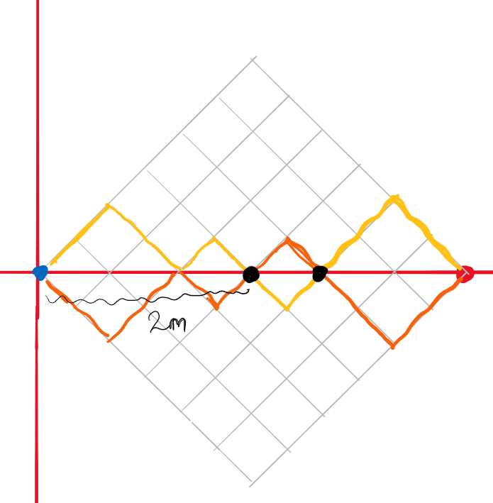
Fig 10: Paths that cross the main diagonal k times. Here, the yellow and symmetric orange paths each cross the red diagonal twice. Note that merely touching it does not count, similar to the Catalan numbers.

To clarify, consider a gambler who starts and ends at a balance of $0, obtaining t heads and t tails. We found that the total number of paths is {2t choose t} and the paths that do not cross $0$ equal 2c_t = 2{2tchoose t}/(t+1)—the same as equation (1), except for a factor of 2 that accounts for paths remaining above or below the $0 threshold (two such symmetric paths illustrated in Figure 3).

Next, we aim to determine the paths that start and end at the $0 mark while crossing the $0 line exactly k times. Let’s denote the number of such paths as r_{k,t}. Clearly, we have r_{0,t}=2c_t (for c_t as defined in equation (1)).

#### 5.1 A Recurrence

Initially, we can derive a recurrence for the r_{k,t} terms by considering the first instance in the path where it crosses the x-axis. This is defined as the first segment of the gambler’s journey, which must occur on 2m tosses (it must be even since the gambler must have an equal number of heads and tails). The number of ways to accomplish this is simply c_m. Following this, the second segment of the gambler’s journey initiates, leaving (2t-2m) tosses remaining while necessitating crossing the main diagonal (k-1) more times to meet the criteria. The number of ways to achieve this is defined as r_{k-1,t-m}. The total ways to complete the journey combine the number of ways to finish the first section with the number of ways to finish the second section. However, this assumes paths crossing the x-axis after m tails. For the total paths, m can vary from 1 to n-1, so we sum over all possibilities to obtain:

Eq (14): The recurrence involving r_{k,t}.

#### 5.2 The Generating Function

Similar to before, let’s define the generating function, R_{k}(z):

Eq (12): Generating function for the r_{k,t} sequence.

Notably, we begin now with t=1, unlike the generating function C_l(z). This adjustment arises because r_{0,t}=0 (0 tails imply 0 heads; if no tosses occur, crossing the main diagonal k times is impossible).

The case where we cross the main diagonal k=0 times is simply the paths we’ve analyzed previously, and the generating function for that scenario should be straightforward:

Eq (13): Generating function for the simple case. The presence of -1 at the end arises from the sequence beginning at t=1, not t=0 as before.

Next, let’s extend this to k=1. By leveraging our earlier observations from the recurrence in equation (14):

Continuing from our earlier conclusion that r_{0,t}=2c_t, and utilizing the index-switching technique applied in equation (4), we obtain:

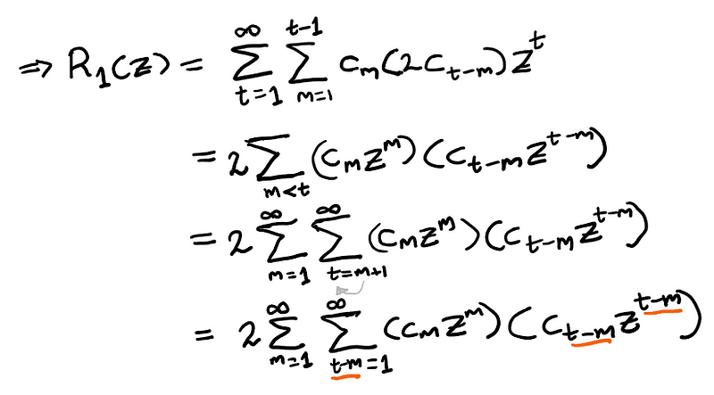
Now, re-index t-m=s and apply the findings from equation (13) to separate the summations, expressed in terms of the previously encountered generating functions:

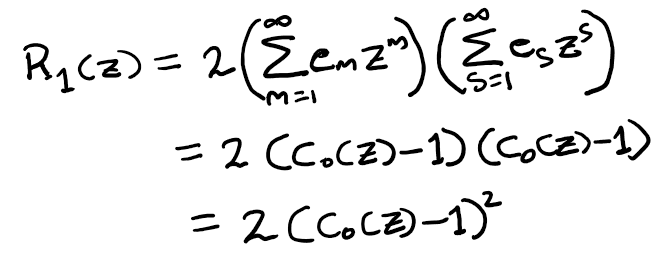
By repeating this entire procedure k-1 times, we derive:

Eq (15): Obtaining the overall generating function for r_{k,t}.

From equation (10), where we established a relationship for C_0(z), we have:

Eq (16): Closed form expression for the r_{k,n} series; the number of paths that cross the main diagonal exactly k times.

It’s important to note that r_{k,n}=0 if n<k, as it would be impossible to cross the diagonal k times if the path length isn’t sufficient. The mathematical concepts presented herein were adapted from various sources.

6. Next Questions

One should always strive to ask the next question. Here are several additional generalizations, all of which yield elegant expressions:

• The number of paths that remain below a specified level.
• The number of paths that are confined between two levels.
• The number of paths that cross a specific level k times.